Fundamental Basics
Contents
\(\begin{align} \newcommand{transp}{^\intercal} \newcommand{F}{\mathcal{F}} \newcommand{Fi}{\mathcal{F}^{-1}} \newcommand{inv}{^{-1}} \newcommand{stochvec}[1]{\mathbf{\tilde{#1}}} \newcommand{argmax}[1]{\underset{#1}{\mathrm{arg\, max}}} \newcommand{argmin}[1]{\underset{#1}{\mathrm{arg\, min}}} \end{align}\)
Computational Imaging
Fundamental Basics#
Content#
Optics
Illumination
Image acquisition and image formation process
Optics#
Conventional imaging: produce sharp image of scene on image plane.
interact(lambda i: showFig('figures/2/imaging_pinhole_lens_',i,'.svg',800,40), i=widgets.IntSlider(min=(min_i:=1),max=(max_i:=4), step=1, value=(max_i if book else min_i)))
<function __main__.<lambda>(i)>
Conventions:
Camera coordinate system \((x^\mathrm{c}, y^\mathrm{c}, z^\mathrm{c})\) equals world coordinate system \((x^\mathrm{w}, y^\mathrm{w}, z^\mathrm{w})\), hence only camera coordinate system is used.
Points of the observed scene are called object points and are denoted by \(\mathbf{p}^\mathrm{c}=(p^\mathrm{c}_x, p^\mathrm{c}_y, p^\mathrm{c}_z)\).
Points on the image plane are denoted by \(\mathbf{p}^\mathrm{b}=(p^\mathrm{b}_x, p^\mathrm{b}_y)\).
Pinhole camera#
In the case of a pinhole camera, the correspondence between an object point \(\mathbf{p}^\mathrm{c}\) and an image point \(\mathbf{p}^\mathrm{b}\) is obtained via the intercept theorem:
\(\begin{align} \frac{p^\mathrm{c}_x}{p^\mathrm{c}_z} = - \frac{p^\mathrm{b}_x}{b}\,, \end{align}\)
with image distance \(b\).
Analogously it is:
\(\begin{align} \frac{p^\mathrm{c}_y}{p^\mathrm{c}_z} = - \frac{p^\mathrm{b}_y}{b}\,. \end{align}\)
Hence:
\(\begin{align} \begin{pmatrix}p^\mathrm{b}_x \\ p^\mathrm{b}_y \end{pmatrix} = -\frac{b}{p^\mathrm{c}_z}\begin{pmatrix} p^\mathrm{c}_x \\ p^\mathrm{c}_y \end{pmatrix} \,. \end{align}\)

Advantages and disadvantages of pinhole cameras:
Advantages:
Easy principle
Infinite focus
Disadvantages:
Images slightly blurry and
system’s low light efficiency (both caused by the small pinhole)
Thin lens camera#
Common cameras employ a lens to collect light and focus it on the sensor. Even lens systems consisting of multiple lenses can be described via the so-called thin lens camera model, where the lens is characterized by its focal length \(f\) and its diameter \(d\).

Principal ray: Connects \(\mathbf{p}^\mathrm{c}\) and \(\mathbf{p}^\mathrm{b}\) and runs through the center of the lens.
Parallel rays: Connect \(\mathbf{p}^\mathrm{c}\) and \(\mathbf{p}^\mathrm{b}\) and run parallel to the optical axis on one side of the lens and cross the optical axis on the other side of the lens at its focal point, i.e., at a distance of \(f\) from the lens.
The correspondence between the focal length \(f\), the distance \(g\) of the plane of focus and the image distance \(b\) is given by the so-called thin lens formula:
\(\begin{align} \frac{1}{f}=\frac{1}{g}+\frac{1}{b}\,. \end{align}\)
If the thin lens equation is met and if \(p^\mathrm{c}_z = g\), the object point is considered to be located in the plane of focus.
The magnification \(V\) of the system is given by:
\(\begin{align} V = \frac{\vert p^\mathrm{b}_y \vert}{\vert p^\mathrm{c}_y \vert} \,. \end{align}\)
Directional information is lost#
The sensor pixel at the position \(\mathbf{p}^\mathrm{b}\) receives the whole light bundle, i.e., it integrates over all directions of incidence of the incident light and the directional information is lost.
Defocus#
The following happens, if the image plane is not located at the image distance \(b\) (calculated via the thin lens formula):

The light bundle does not converge in a point on the image sensor but is distributed over an area called the circle of confusion.
If the area of the circle of confusion exceeds the area of a single pixel of the sensor, the image starts to appear blurred.

The depth of focus or depth of field denotes the distance at the object side of the lens by which an object point can be moved out of the plane of focus so that the circle of confusion of its converging light bundle still remains below the area of one sensor element.
If the sensor elements could resolve the direction of incidence of the incident light rays, a sharp image could be reconstructed by combining the respective rays from each sensor to create a synthesized image (more later at light field imaging).
Aperture#
The aperture of an optical system is the optical or mechanical element mostly limiting, i.e. blocking, the captured light bundle.
Captured bright object points lying outside the plane of focus form an image of the aperture on the sensor plane. This effect is called Bokeh and is sometimes used as a stylistic element in photography.
Stopping down, i.e., reducing the size of the aperture, reduces the amount of light captured while decreasing the size of the circle of confusion what increases the depth of field:

The pattern of the aperture can also be made controllable, e.g., by employing a transmissive LCD. This gives further control over the image formation process and is the key ingredient to coded aperture imaging (more later).
Acquisition of the light’s direction of propagation#
When imaging with a lens, light rays intersect the image-side focal plane (i.e., the plane located with a distance of \(f\) to the lens and being oriented perpendicularly to the optical axis) at positions which correspond to the deflection angles of those rays w.r.t. the optical axis:

Objects located at optical infinity, i.e., at a distance \(g \gg f\), will result in collimated light beams, i.e., light rays propagating parallel to each other. The corresponding image points are located on the image-side focal plane:

The distance \(\delta_\alpha\) of the location of the intersection of the converging ray bundle with the focal plane now only depends on the object-side angle of the parallel light beams w.r.t. to the optical axis and on the focal length \(f\):
\(\begin{align} \delta_\alpha=f\cdot \tan(\alpha)\,. \end{align}\)

This setup transforms directional information about the light’s direction of propagation into spatial information (i.e., the distance \(\delta_\alpha\)). By placing a sensor in the focal plane, this information can be captured. Since all rays of the collimated bundle are focused to the same position on the focal plane, any spatial information about the single light rays is lost and has to be obtained by other means.
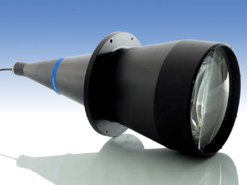
Example of directional filtering: Telecentric imaging#
Just shown: Spatial positions on the image-side focal plane correspond to directional information about captured light rays.
Spatial filters placed in the image-side focal plane act as directional filters w.r.t. the captured light rays.
Frequently used filter: Pinhole centered at the optical axis.

Such a pinhole is called a telecentric stop and allows only such rays to reach the sensor which propagate (approximately) parallel to the optical axis on the object side.
By this means, the magnification \(V\) of the system is independent of the distance of image objects to the lens.
Important: Since the opening of the telecentric stop allows ray bundles of a certain size to reach the sensor, the system is also affected by defocus effects.
Let’s play around with optics#
https://phydemo.app/ray-optics/simulator/?en
Or in short: https://s.fhg.de/optics-simulator
Illumination#
Physical principles of illumination#
Two main different physical effects can be exploited to emit light:
Thermal radiation
A certain material is heated (energy supply) and therefore emits light.
Examples: Halogen lamps, fluorescent lamps, metal vapor lamps, xenon short-arc lamps.Luminescsent radiation
Potential energy is directly transformed into light.
Examples: Gas-discharge lamps, light-emitting diodes (LEDs) and lasers.
The emitted spectrum heavily depends on the employed technology.
Illumination techniques:#
Point light source#
Concept:
An infinitely small point shaped light source emitting light uniformly in all directions.

Realization:
LEDs (ultra bright ones).
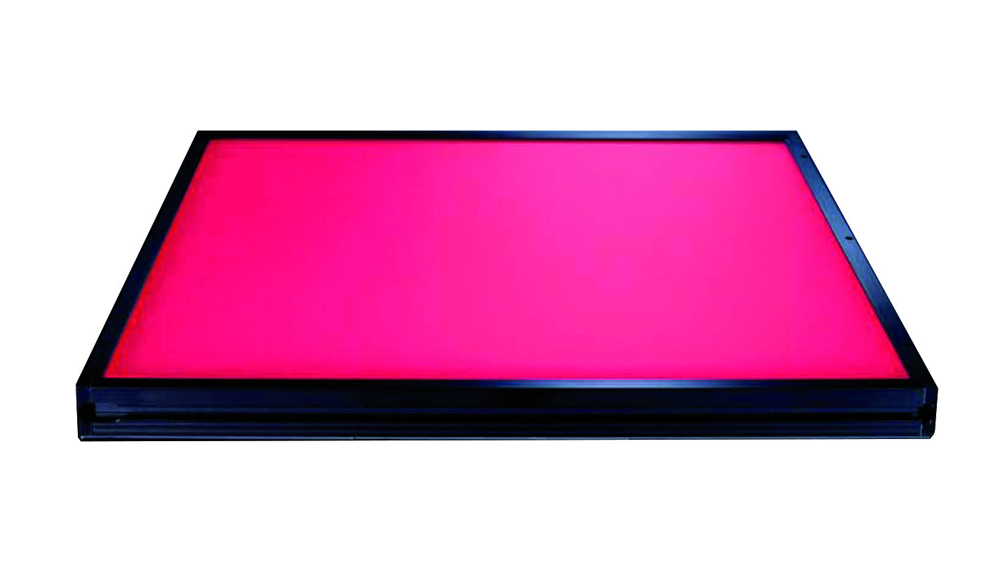
Area light source#
Concept:
Finite size area of which each point emits beams of light of a certain spectrum uniformly into all directions of the respective half-space.

Realization:
Multiple LEDs arranged in a dens grid behind a diffuser.
Programmable area light sources#
Concept:
Similar to the area light source extended by a controllable spatial pattern of the emitted spectrum (including its intensity).

Realization:
Computer display / projector.
Note: It is also possible to control the direction of propagation of the emitted light as will be shown now for a special case (more later at light field illumination).
Telecentric illumination#
Concept:
Similar to telecentric imaging light sources can be adapted to only emit light rays that propagate approximately parallel to each other.

Realization: Point light source placed in the focal point of a lens, i.e., with \(\delta_\alpha = 0\), so that
\(\begin{align} 0 = f\cdot \tan(\alpha) \Leftrightarrow \alpha = 0^\circ\,. \end{align}\)
Note: It is also possible to realize a telecentric light source with a spatially controllable pattern.
Image acquisition and image formation process#
Image acquisition model#
For the scope of this course (except stated otherwise), the image acquisition process is assumed to follow this model:

\(L\) : Light field which illuminates the scene and which is generated by the illumination device.
\(L'\): Light field modulated by the scene.
\(f_\mathrm{phys}(L,\mathbf{\unicode{x3BE}}_\mathrm{geom})\): Modulation, involving geometric parameters \(\mathbf{\unicode{x3BE}}_\mathrm{geom}\) (e.g., orientation of the scene).
\(\mathbf{g}\): Digital image resulting from the sensor capturing a section of \(L'\).
\(f_\mathrm{sens}(L',\mathbf{\unicode{x3BE}}_\mathrm{sens})\): Image acquisition, involving parameters \(\mathbf{\unicode{x3BE}}_\mathrm{sens}\) (e.g., alignment, orientation and acquisition parameters of the sensor).
\(\mathbf{g'}\): Processed image.
\(f_\mathrm{proc}(\mathbf{g},\mathbf{\unicode{x3BE}}_\mathrm{proc})\): Image processing algorithms with parameters \(\mathbf{\unicode{x3BE}}_\mathrm{proc}\,\).
Image signals \(\mathbf{g}\) will typically be modelled as functions
\(\begin{align}
\mathbf{g}:\Omega \rightarrow \mathbb{R}^c\,,\quad \Omega \subseteq \mathbb{R}^2
\end{align}\)
defined over a two-dimensional support \(\Omega\) and yielding \(c\)-channel image values \(\mathbf{g}\) for every position \(\mathbf{x}\):
\(\begin{align}\mathbf{g}(\mathbf{x})=\begin{pmatrix}
g_1(\mathbf{x})\\ g_2(\mathbf{x}) \\ \vdots \\ g_c (\mathbf{x})
\end{pmatrix}\,, \quad \mathrm{with} \quad \mathbf{x} =
\begin{pmatrix}
x \\ y
\end{pmatrix}\,.\end{align}\)
Note: Digital image signals are usually not continuous, neither w.r.t. their support nor w.r.t. their values.
Framework system theory#
The whole set of imaging components (illumination, lenses, sensor, algorithms, etc.) can be considered as a system \(\mathscr{S}\).
The system transforms an input signal \(\mathbf{f}(\mathbf{x})\) to an output signal \(\mathbf{k}(\mathbf{x})\):
\(\begin{align} \mathbf{k}(\mathbf{x})=\mathscr{S}\lbrace \mathbf{f}(\mathbf{x}) \rbrace \,. \end{align}\)

An important type of systems are so-called linear shift invariant (LSI) systems for which the following two properties hold:
Linearity#
Given two signals \(\mathbf{f}(\mathbf{x}), \mathbf{f}'(\mathbf{x})\) and two constants \(a, a'\), a system \(\mathscr{S}\) is called linear if
\(\begin{align} \mathscr{S}\lbrace a\, \mathbf{f}(\mathbf{x}) + a'\, \mathbf{f}'(\mathbf{x})\rbrace=a\, \mathscr{S}\lbrace \mathbf{f}(\mathbf{x})\rbrace + a'\, \mathscr{S}\lbrace \mathbf{f}'(\mathbf{x}) \rbrace\,. \end{align}\)
Shift invariance#
A system \(\mathscr{S}\) is called shift invariant if
\(\begin{align} \mathscr{S}\lbrace \mathbf{f}(\mathbf{x}-\mathbf{x}_0) \rbrace = \mathbf{k}(\mathbf{x}-\mathbf{x}_0) \quad \mathrm{with} \quad \mathbf{k}(\mathbf{x})=\mathscr{S}\lbrace\mathbf{f}(\mathbf{x})\rbrace \,. \end{align}\)
The effect of an LSI system on a signal can be comfortably studied by means of its impulse response, which will be explained after the introduction of some necessary definitions.
Example#
Consider a spatial modulation, i.e., the system \(\mathscr{S}\lbrace g(x) \rbrace = g(x) \cdot m(x) = k(x)\).
Then \(k(x-x_0) = g(x-x_0) \cdot m(x-x_0)\) but
\( \mathscr{S}\lbrace g(x-x_0) \rbrace = g(x-x_0) \cdot m(x)\).
Hence, \(\mathscr{S}\lbrace \cdot \rbrace\) is not shift invariant and therefore not an LSI system.
Dirac delta function#
Note: For the sake of simplicity, the scalar case is considered at first.
The Dirac delta function \(\delta(x)\) is defined via its effect when being used as an integral kernel together with an arbitrary function \(f(x)\):
\(\begin{align}
\int\limits^\infty_{-\infty} \delta(x-x_0)f(x) \mathrm{d}x = f(x_0) \quad \mathrm{with}\, f(x)\, \mathrm{continuous\, at}\, x_0\,.
\end{align}\)
\(\Rightarrow\) it extracts the value of \(f(x)\) at the position \(x_0\).
Assuming \(f(x)\equiv 1\) immediately implies
\(\begin{align} \int\limits^\infty_{-\infty} \delta (x) \mathrm{d}x = 1\,. \end{align}\)
The Dirac delta function can be imagined as a very narrow, impulse-shaped function with an integral of \(1\). It can be approximated via:
\(\begin{align} \delta_\varepsilon (x):=\frac{1}{\varepsilon}\,\mathrm{rect}(x,\varepsilon) \end{align}\)
with the rectangular function
\(\begin{align} \mathrm{rect}(x,\varepsilon):=
\begin{cases}
1 \quad \mathrm{if}\, \vert x \vert < \frac{\varepsilon}{2}\,, \\
0 \quad \mathrm{otherwise}\,,
\end{cases} \end{align}\)
with \(\varepsilon\) denoting the width of the impulse.
For \(\varepsilon \rightarrow 0\) it holds:
\(\begin{align}
\lim_{\varepsilon \rightarrow 0} \int\limits^\infty_{-\infty} \delta_\varepsilon(x-x_0)f(x)\mathrm{d}x=f(x_0)=\int\limits^\infty_{-\infty} \delta(x-x_0)f(x) \mathrm{d}x \quad
\end{align}\)
\(\mathrm{with}\, f(x)\, \mathrm{continuous\, at}\, x_0\,,\)
since \(f(x) \approx f(x_0)\) for a sufficiently small neighborhood of \(\varepsilon\) around \(x_0\) because of the continuity of \(f(x)\) in \(x_0\), leading to
\(\begin{align} \delta_\varepsilon(x)\xrightarrow{\varepsilon \rightarrow 0} \delta(x)\,. \end{align}\)
Visualization of the Dirac delta function#
def rect(x,eps):
    if np.linalg.norm(x) < (eps/2.0):
        return 1
    else:
        return 0
def diracEps(x,eps):
    return (1.0/eps) * rect(x,eps)
def plotDiracEps(eps):
    factor = 100.0
    xs = np.arange(-5, 5, 1/factor, dtype=np.float32)
    ys = [diracEps(x,eps) for x in xs]
    plt.clf()
    plt.plot(xs, ys)
    print("Integral: " + str(np.sum(ys)/factor))
plt.figure()
interact(plotDiracEps, eps=widgets.FloatSlider(min=(min_i:=0.01),max=(max_i:=2.0), step=0.1, value=(min_i if book else max_i)))
<Figure size 432x288 with 0 Axes>
<function __main__.plotDiracEps(eps)>
2D Dirac delta function#
The two-dimensional Dirac delta function is defined as
\(\begin{align}
\int\limits^\infty_{-\infty}\int\limits^\infty_{-\infty}\delta (\mathbf{x}-\mathbf{x_0})f(\mathbf{x})\mathrm{d}\mathbf{x}=f(\mathbf{x}_0)\quad \mathrm{with\,}f(\mathbf{x})\,\mathrm{continuous\,at\,}\mathbf{x}_0\,.
\end{align}\)
The same properties hold as for the one-dimensional case.
Convolution#
The convolution \(f(x)* h(x)\) of two functions \(f(x),h(x)\) is defined as:
\(
\begin{align}
f(x)* h(x):= \int\limits^\infty_{-\infty}f(\alpha)h(x-\alpha)\mathrm{d}\alpha=\int\limits^\infty_{-\infty}f(x-\alpha)h(\alpha)\mathrm{d}\alpha\,.
\end{align}
\)
Convolving an arbitrary function \(f(x)\) with \(\delta(x-x_0)\) corresponds to shifting \(f(x)\) by \(x_0\):
\(\begin{align}
f(x)*\delta(x-x_0)=\int\limits^\infty_{-\infty}f(\alpha)\delta(\underbrace{x-x_0-\alpha}_{=\,0\, \Leftrightarrow\, \alpha\, =\, x-x_0})\mathrm{d}\alpha=f(x-x_0)\,.
\end{align}
\)
Hence, for \(x_0=0:\quad f(x)*\delta(x)=f(x)\,.\)
2D convolution#
The two-dimensional convolution of two functions \(f(\mathbf{x}), h(\mathbf{x})\) is denoted by the \(**\)-operator and is defined as follows:
\(\begin{align}
f(\mathbf{x})**h(\mathbf{x}) := \int\limits^\infty_{-\infty}\int\limits^\infty_{-\infty} f\left((\alpha,\beta)^\intercal\right)h\left( (x-\alpha, y-\beta)^\intercal \right)\mathrm{d}\alpha\, \mathrm{d}\beta\,.
\end{align}\)
Play around with convolutions#
https://lpsa.swarthmore.edu/Convolution/CI.html
In short: https://s.fhg.de/convolution
Impulse response of an LSI system#
The response of an LSI system \(\mathscr{S}\lbrace \cdot \rbrace\) to an input signal \(f(x)\) can be expressed using a convolution integral:
\(\begin{align}
\mathscr{S}\lbrace f(x)\rbrace =
\mathscr{S}\lbrace f(x) * \delta(x) \rbrace &=
\mathscr{S} \left\lbrace \int\limits^\infty_{-\infty} f(\alpha)\delta(x-\alpha)\mathrm{d}\alpha \right\rbrace \\ &=
\int\limits^\infty_{-\infty}f(\alpha)\underbrace{\mathscr{S}\lbrace\delta(x-\alpha)\rbrace}_{h(x-\alpha)}\mathrm{d}\alpha \\ &=
f(x)*h(x)\,.
\end{align}\)
The response \(h(x)=\mathscr{S}\lbrace \delta(x) \rbrace\) of \(\mathscr{S}\lbrace \cdot \rbrace\) to the input \(\delta(x)\) is called the impulse response of \(\mathscr{S}\lbrace \cdot \rbrace\).
An LSI system is completely characterized by its impulse response \(h(x)\).
Example: Impulse response of a defocused optical imaging system#
For a defocused optical imaging system (see 2.1.2.1), object points from the observed scene are mapped to circles of confusion on the sensor.
Such an optical system can be interpreted and handled as an LSI system.
Hence, the impulse response function \(h(\mathbf{x})\) is sufficient for the complete characterization of the system.
Acquiring \(h(\mathbf{x})\)#
One way to acquire \(h(\mathbf{x})\), is to present an impulse-shaped input to the system and record its answer.
With respect to optical systems, an impulse corresponds to a scene having only a single bright point centered at the optical axis.
In the domain of optics, \(h(\mathbf{x})\) is often also denoted as the so-called point spread function (PSF), as will be illustrated by the upcoming example.

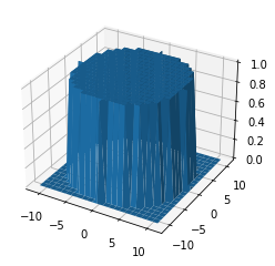
The impulse response \(h(\mathbf{x})\) will have the shape of a two-dimensional \(\mathrm{rect}\)-function:
\(\begin{align}
h(\mathbf{x}) = \mathrm{rect}\left( \Vert \mathbf{x} \Vert, \varepsilon \right)\,,
\end{align}\)
sometimes also denoted as the so-called pillbox function (looks like a round box for drugs).
To simulate the output of the system for a scene, e.g., given as a grayscale image \(g(\mathbf{x})\), it is sufficient to calculate \(g(\mathbf{x})**\,h(\mathbf{x})\) as will be shown in the following example.
def createPillobxResponse(r):
    X,Y = np.meshgrid(np.arange(-r-1,r+2,1), np.arange(-r-1,r+2,1))
    psf = np.zeros_like(X)
    psf[np.sqrt(X**2+Y**2) <= r] = 1
    return psf, X, Y
psf, X, Y = createPillobxResponse(10)
fig, ax = plt.subplots(subplot_kw={"projection": "3d"})
surf = ax.plot_surface(X, Y, psf)
plt.show()
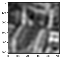
img = cv2.cvtColor(plt.imread('figures/2/input_Cam020.png'), cv2.COLOR_RGB2GRAY)
plt.figure()
imshow(img, cmap='gray')
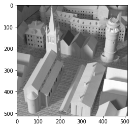
def defocusExample(r):
    psf, _, _ = createPillobxResponse(r)
    res = ndimage.convolve(img, psf, mode='constant', cval=0.0)
    imshow(res, cmap='gray')
plt.figure()
interact(defocusExample, r=widgets.IntSlider(min=(min_i:=0),max=(max_i:=10), step=1, value=(max_i if book else min_i)))
<Figure size 432x288 with 0 Axes>
<function __main__.defocusExample(r)>
Fourier transform#
Fourier series, trigonometric form#
Every periodic function \(g(x)\) with a periodic interval \(\left[0, L\right]\) can be expressed as a series of weighted sine functions and cosine functions via the so-called Fourier series synthesis:
\(\begin{align}
g(x) = a_0 + \sum\limits^\infty_{f=1} \left(a_f \cos \left( \frac{2\pi f x}{L} \right) + b_f \sin \left(\frac{2\pi f x}{L} \right)\right)\,,
\end{align}\)
with \(a_f\) and \(b_f\) denoting the Fourier series coefficients.
The Fourier series coefficients are obtained via the Fourier series analysis:
\(\begin{align}
a_0 &= \frac{1}{L} \int\limits^L_0 g(x)\mathrm{d}x \\
a_f &= \frac{2}{L} \int\limits^L_0 g(x) \cos\left(\frac{2\pi f x}{L}\right) \mathrm{d}x \\
b_f &= \frac{2}{L} \int\limits^L_0 g(x) \sin\left(\frac{2\pi f x}{L}\right) \mathrm{d}x
\end{align}\)
The index \(f\) denotes the frequency of the approximating oscillations with respect to the periodic interval \(\left[0,L\right]\) of \(g(x)\).
Higher \(f\) correspond to higher frequencies which encode fine details of \(g(x)\).
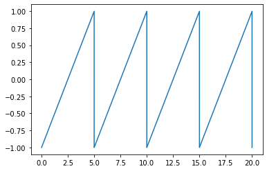
Example: Trigonometric Fourier series calculation#
L=20
freq=4
samples=10000
xs = (np.linspace(0,L,samples,endpoint=True))
gs = sig.sawtooth(2*np.pi*xs*freq/L,)
plt.figure()
plt.plot(xs, gs)
[<matplotlib.lines.Line2D at 0x231676fc940>]
a0 = 1/L * simpson(gs,xs)
an = []
bn = []
for i in range(1,110):
    an.append((2.0/L)*simpson(gs*np.cos(2*np.pi*i*xs/L) ,xs))
    bn.append((2.0/L)*simpson(gs*np.sin(2*np.pi*i*xs/L) ,xs))
def reconstrTrigFourier(terms):
    a0 = 1/L * simpson(gs,xs)
    an = []
    bn = []
    for i in range(1,terms):
        an.append((2.0/L)*simpson(gs*np.cos(2*np.pi*i*xs/L) ,xs))
        bn.append((2.0/L)*simpson(gs*np.sin(2*np.pi*i*xs/L) ,xs))

    gs2 = np.zeros_like(xs)
    gs2 = gs2 + a0
    for i in range(0,len(an)):
        gs2 = gs2 + an[i]*np.cos(2*np.pi*xs/L*(i+1)) + bn[i]*np.sin(2*np.pi*xs/L*(i+1))

    plt.clf()
    plt.plot(xs,gs2)
    plt.plot(xs,gs)
plt.figure()
interact(reconstrTrigFourier, terms=widgets.IntSlider(min=(min_i:=1),max=(max_i:=100), step=4, value=(max_i if book else min_i)))
<Figure size 432x288 with 0 Axes>
<function __main__.reconstrTrigFourier(terms)>
Fourier series, exponential form#
The concept of Fourier series can be further simplified and compacted by making use of complex numbers \(a+b\,\mathrm{j} \in \mathbb{C}\) with the imaginary unit \(\mathrm{j}\).
Key ingredient to the following considerations is the so-called Euler’s formula:
\(\begin{align}
\mathrm{e}^{\,\mathrm{j}x}&= \cos(x)+\mathrm{j}\,\sin(x)\,,\\
\mathrm{e}^{\,-\mathrm{j}x}&= \cos(x)-\mathrm{j}\,\sin(x)\,.
\end{align}\)
The Fourier synthesis then simplifies to
\(\begin{align}
g(x)=\sum\limits^{+\infty}_{f=-\infty} c_f \exp\left(\frac{\mathrm{j}2\pi f x}{L}\right)\,,
\end{align}\)
with \(c_f\) denoting the complex Fourier coefficients.
The complex Fourier coefficients are obtained via the more compact complex Fourier analysis:
\(\begin{align}
c_f = \frac{1}{L} \int\limits^L_0 g(x)\exp\left(\frac{-\mathrm{j}2\pi f x}{L}\right)\mathrm{d}x
\end{align}\)
The coefficients are symmetric in the way that \(c_i = c^*_{-i}\) with \(^*\) denoting the complex conjugate. Hence, all the imaginary parts cancel out during the synthesis of a real-valued input signal \(g(x)\).
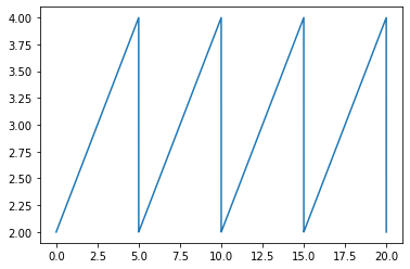
Example: Exponential Fourier series calculation#
L=20.0
freq=4
samples=10000
xs = (np.linspace(0,L,samples,endpoint=True))
gs = sig.sawtooth(2*np.pi*xs*freq/L,)+3
plt.figure()
plt.plot(xs, gs)
[<matplotlib.lines.Line2D at 0x23167749730>]
def reconstrExpFourier(terms):
    fs = np.arange(-1*terms,terms+1)
    cn = np.zeros(len(fs),dtype='complex128')
    for i in range(0,len(fs)):
        cn[i]=((1.0/L)*simpson(gs*np.exp(-1j*2*np.pi*fs[i]*xs/L),xs))

    gs2 = np.zeros_like(xs)
    for i in range(0,len(fs)):
        gs2 = gs2 + cn[i]*np.exp(1j*2*np.pi*fs[i]*xs/L)

    plt.clf()
    plt.plot(xs,np.real_if_close(gs2))
    plt.plot(xs,gs)
plt.figure()
interact(reconstrExpFourier, terms=widgets.IntSlider(min=(min_i:=1),max=(max_i:=100), step=1, value=(max_i if book else min_i)))
<Figure size 432x288 with 0 Axes>
<function __main__.reconstrExpFourier(terms)>
Here you can find a great applet to play around with Fourier series: https://www.falstad.com/fourier/
Let’s play the wave game!#
https://phet.colorado.edu/sims/html/fourier-making-waves/latest/fourier-making-waves_all.html
In short: https://s.fhg.de/wave-game
Fourier transform#
The Fourier transform transforms a nearly arbitrary, usually real-valued function \(g(x)\) into a complex-valued function \(G(f):\mathbb{R}\rightarrow \mathbb{C}\) with frequency \(f\):
\(\begin{align}
G(f):=\int\limits^\infty_{-\infty}g(x) \exp (-\mathrm{j}2\pi f x)\,\mathrm{d}x=:\mathscr{F}\lbrace g(x) \rbrace\,,
\end{align}\)
which is also called the spectrum of \(g(x)\).
The inverse transform is given by:
\(\begin{align}
g(x)=\int\limits^\infty_{-\infty}G(f)\exp(\mathrm{j}2\pi f x)\,\mathrm{d}f=:\mathscr{F}^{-1}\lbrace G(f) \rbrace\,.
\end{align}\)
Since \(G(f)\in \mathbb{C}\), it can be expressed as
\(\begin{align}
G(f)=\vert G(f) \vert\cdot \exp(\mathrm{j}\varphi(f)) = \mathscr{R}\lbrace G(f) \rbrace + \mathrm{j}\,\mathscr{I}\lbrace G(f) \rbrace\,,
\end{align}\)
with \(\vert G(f) \vert\) denoting the magnitude spectrum, \(\varphi(f)\) denoting the phase spectrum, \(\mathscr{R}\lbrace G(f) \rbrace\) denoting the real part of \(G(f)\) and \(\mathscr{I}\lbrace G(f) \rbrace\) denoting the imaginary part of \(G(f)\).
The variable \(f\) of \(G\) denotes a frequency with respect to spatial positions (not to time!), which is why it is denoted as a spatial frequency with unit \(\left[f\right]=\left[x\right]^{-1}\).
Common naming conventions:
Spatial domain: the domain of \(g(x)\),
Fourier domain or spatial frequency domain: the domain of \(G(f)\).
2D Fourier transform#
The two-dimensional Fourier transform \(G(\mathbf{f}):\mathbb{R}^2\rightarrow \mathbb{C},\, \mathbf{f}=(f_x,f_y)^\intercal\) of a two-dimensional function \(g(\mathbf{x}):\mathbb{R}^2 \rightarrow \mathbb{C},\, \mathbf{x}=(x,y)^\intercal\) is obtained via the following integral transform:
\(\begin{align}
G(\mathbf{f})=\mathscr{F}\lbrace g(\mathbf{x}) \rbrace := \int\limits^\infty_{-\infty}\int\limits^\infty_{-\infty}g(\mathbf{x}) \exp \left(-\mathrm{j}2\pi\,\mathbf{f}^\intercal \mathbf{x} \right) \mathrm{d} \mathbf{x} \,.
\end{align}\)
The inverse transform is given by:
\(\begin{align}
g(\mathbf{x})=\mathscr{F}^{-1}\lbrace G(\mathbf{f}) \rbrace = \int\limits^\infty_{-\infty}\int\limits^\infty_{-\infty} G(\mathbf{f}) \exp\left( \mathrm{j}2\pi\,\mathbf{f}^\intercal \mathbf{x} \right) \mathrm{d}\mathbf{f}\,.
\end{align}\)
Convolution theorem#
Consider the Fourier transform of the convolution of two signals \(g(x), h(x)\):
\(\begin{align}
\mathscr{F}\lbrace g(x) * h(x) \rbrace &= \int\limits^\infty_{-\infty}\int\limits^\infty_{-\infty}g(\alpha)h(x-\alpha)\mathrm{d}\alpha\, \exp\left( -\mathrm{j}2\pi f x \right)\, \mathrm{d} x\\
&= \int\limits^\infty_{-\infty}g(\alpha)\int\limits^\infty_{-\infty}h(x-\alpha)\exp\left( -\mathrm{j}2\pi f x \right)\, \mathrm{d}x\,\mathrm{d} \alpha \,.
\end{align}\)
Now, the substitution \(\beta:= x- \alpha\) yields:
\(\begin{align}
\mathscr{F}\lbrace g(x) * h(x) \rbrace &= \int\limits^\infty_{-\infty}g(\alpha)\int\limits^\infty_{-\infty}h(\beta)\exp\left( -\mathrm{j}2\pi f (\alpha + \beta) \right)\, \mathrm{d}\beta\,\mathrm{d} \alpha \\
&= \underbrace{ \int\limits^\infty_{-\infty} g(\alpha) \exp\left( -\mathrm{j}2\pi f \alpha \right)\, \mathrm{d} \alpha }_{G(f)}\cdot
\underbrace{\int\limits^\infty_{-\infty} h(\beta) \exp\left( -\mathrm{j}2\pi f \beta \right)\, \mathrm{d} \beta}_{H(f)}\,.
\end{align}\)
Hence, the Fourier transform transforms the convolution of two signals into a multiplication of their spectra and vice versa:
\(\begin{align}
g(x)*h(x) &= \mathscr{F}^{-1}\lbrace G(f)\cdot H(f) \rbrace \,, \\
g(x)\cdot h(x) &= \mathscr{F}^{-1}\lbrace G(f) * H(f) \rbrace \,. \\
\end{align}\)
This dualism can be exploited in various ways, e.g., to speed up the calculation of a convolution by performing it as a multiplication in the frequency space (i.e., Fourier domain).
Discrete Fourier transform (DFT)#
The Fourier transform requires unlimited continuous signals what can’t be practically realized in a computer (no unlimited storage).
As a practical approximation, the discrete Fourier transform (DFT) can be employed.
The signal \(g(x)\) is assumed to be sampled at \(N\) positions having an equidistant spacing of \(\Delta x\), i.e., \(x=n \Delta x, n\in\left[0,\ldots,N-1\right]\).
The DFT \(G(f)\) of \(g(x)\) is then obtained via:
\(\begin{align}
G(f) = \sum\limits^{N-1}_{n=0} g(n\Delta x)\exp\left( -\mathrm{j}2\pi \frac{fn}{N} \right) \,.
\end{align}\)
The inverse DFT is calculated as:
\(\begin{align}
g(n\Delta x)\approx \frac{1}{N} \sum\limits^{N-1}_{f=0} G(f) \exp \left( \mathrm{j}2\pi \frac{fn}{N} \right)\,.
\end{align}\)
Illustration of the DFT#
interact(lambda i: showFig('figures/2/dftSpectrum_',i,'.svg',800,60), i=widgets.IntSlider(min=(min_i:=1),max=(max_i:=3), step=1, value=(max_i if book else min_i)))
<function __main__.<lambda>(i)>
Note#
The following two important properties of the DFT can be seen in the last step of the animation:
The DFT implicitly periodically repeats the approximated spectrum.
This has to be taken into account when making use of the convolution theorem, since convolutions performed as multiplications in the Fourier domain (calculated with the DFT) have to be regarded as cyclic.
The center of the extracted window of length \(N\) corresponds to the highest spatial frequencies.
By appropriately swapping the window halves, the correct arrangement can be obtained.
Example: DFT calculation#
L=20.0
freq=4
samples=10001
xs = (np.linspace(0,L,samples,endpoint=True))
xs2 = np.arange(0,samples)
gs = sig.sawtooth(2*np.pi*xs*freq/L,)
plt.figure()
plt.plot(xs, gs)
[<matplotlib.lines.Line2D at 0x231678b0a90>]

cn = np.zeros(samples,dtype='complex128')
for i in range(0,samples):
    cn[i] = np.sum(gs * np.exp(-1j*2*np.pi*xs2*i/samples))
gs2 = np.zeros_like(cn)
for i in range(0,samples):
    gs2[i] = (1.0/samples) * np.sum(cn*np.exp(1j*2*np.pi*xs2*i/samples))
plt.figure()
plt.plot(xs,np.real_if_close(gs2))
plt.plot(xs,gs)
C:\Users\meyjoh\repos\vlcompimg\compimg\lib\site-packages\matplotlib\cbook\__init__.py:1333: ComplexWarning: Casting complex values to real discards the imaginary part
  return np.asarray(x, float)
[<matplotlib.lines.Line2D at 0x2316785c520>]

Note#
In practice, one would employ one of the existing, highly optimized libraries to perform the DFT calculation, e.g., the numpy.fft module.
Let’s play around with Fourier transforms#
https://monman53.github.io/2dfft/
Or in short: https://s.fhg.de/fourier
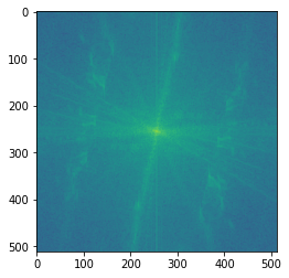
Example Fourier transform-based image filtering#
plt.figure()
plt.imshow(img, cmap='gray')
<matplotlib.image.AxesImage at 0x23167594160>

img_fft = np.fft.fft2(make_odd_shapes(img))
plt.figure()
img_fft = np.fft.fftshift(img_fft)
plt.imshow(np.log(np.abs(img_fft)))
<matplotlib.image.AxesImage at 0x231640b9fd0>
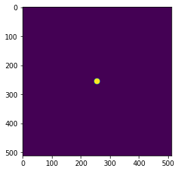
r = 10
psf, _, _ = createPillobxResponse(r)
psf = pad_like(psf, img_fft)
plt.figure()
plt.imshow(psf)
<matplotlib.image.AxesImage at 0x2316783e160>
img_filtered_fft = img_fft * psf
plt.figure()
plt.imshow(np.log(np.abs(img_filtered_fft)))
<ipython-input-39-6a3f463803e5>:3: RuntimeWarning: divide by zero encountered in log
  plt.imshow(np.log(np.abs(img_filtered_fft)))
<matplotlib.image.AxesImage at 0x231690383d0>
res_img = np.fft.ifft2(np.fft.ifftshift(img_filtered_fft))
plt.figure()
plt.imshow(np.real(res_img), cmap='gray')
<matplotlib.image.AxesImage at 0x231696c4730>
def fourier_filtering(r):
    psf, _, _ = createPillobxResponse(int(r*img_fft.shape[0]/2))
    psf = pad_like(psf, img_fft)
    img_filtered_fft = img_fft * psf
    res_img = np.fft.ifft2(np.fft.ifftshift(img_filtered_fft))
    plt.figure()
    plt.imshow(np.real(res_img), cmap='gray')
interact(lambda i: fourier_filtering(i), i=widgets.FloatSlider(min=(min_i:=0.02),max=(max_i:=0.5), step=0.02, value=(0.08 if book else min_i)))
<function __main__.<lambda>(i)>
Analysis of optical systems in Fourier space#
We learnt: The effect of an LSI on an input signal \(g(x)\) can be obtained via convolution with the system’s PSF \(h(x)\):
\(\begin{align} k(x) = \mathscr{S} \left\{ g(x) \right\} = g(x) * h(x) \end{align}\)
According to the convolution theorem of the Fourier transform it is:
\(\begin{align} \F \left\{ k(x) \right\} = K(f) = G(f) \cdot H(f) \,. \end{align}\)
So the Fourier transform of the PSF determines to what extent every spatial frequency is propagated through the LSI.
Optical transfer function#
The optical transfer function \(\mathrm{OTF}(f)\) is defined as the Fourier transform of the PSF \(h(x)\):
\(\begin{align} \mathrm{OTF}(f) := \F \left\{ h(x) \right\} \,. \end{align}\)
Modulation transfer function#
Since the \(\mathrm{OTF}\) is typically complex-valued and hence hard to visualize, one often relies on the modulation transfer function \(\mathrm{MTF}(f)\) which is the absolute value of the \(\mathrm{OTF}\):
\(\begin{align} \mathrm{MTF}(f) := \left| \mathrm{OTF} (f) \right| \,. \end{align}\)
For visualizations the MTF is often also normalized w.r.t. the direct component (i.e., \(\mathrm{MTF}(0)\)).
Example modulation transfer functions#
In-focus optical system#
The PSF of an optical system producing a sharp image is just \(\delta(x)\), i.e., it is
\(\begin{align} \mathscr{S}\left\{ g(x) \right\} = g(x) \,. \end{align}\)
Hence, the OTF has to be equal to one, i.e., \(\mathrm{OTF}(f) \equiv 1\), since the input signal is left untouched by the system.
This implies \(\mathrm{MTF}(f) \equiv 1\).
Defocused optical system#
interact(lambda i: defocusMTF(i), i=widgets.IntSlider(min=(min_i:=0),max=(max_i:=10), step=1, value=(3 if book else min_i)))
<function __main__.<lambda>(i)>